
Image classification usually ends with a fixed list of class scores. Metric learning offers another route: learn an embedding, compare it with labeled reference images, and infer a label from the nearest useful examples. In part one of our bird classification series, we train that kind of representation using PyTorch and triplet-margin loss.
The companion repository contains the dataset loader, a modified AlexNet, a training notebook, visualization tools, and the indexing workflow used in part two. The video title refers to the bird dataset available at the time; inspect the downloaded dataset's actual class list instead of hard-coding a species count from an old title.
Learn relationships instead of only a class head
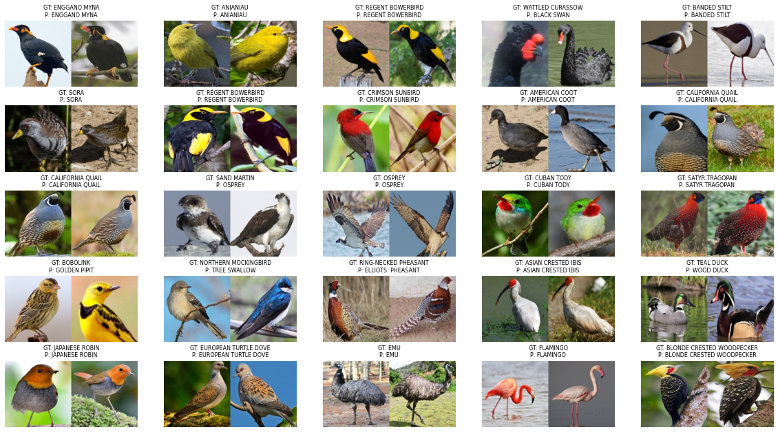
A useful embedding places related images near one another according to the chosen similarity measure. For this experiment, the relationship is shared bird species. The model is trained to separate examples with different labels while drawing same-label examples closer in the learned representation.
This gives the application a gallery to inspect. A prediction can return the reference images that support it, rather than only a class score. Adding gallery examples does not require changing the embedding dimension. That flexibility is useful, but it does not guarantee correct recognition of new species: performance still depends on whether the learned visual features transfer to those examples.
A small embedding head on AlexNet
The project's model wrapper uses AlexNet and replaces its classifier with a linear layer producing the requested embedding size. The training notebook uses 128-pixel inputs and a 64-dimensional output, starts from pretrained weights, and normalizes input channels with the recorded mean and standard deviation.
These choices make the experiment easy to inspect. They are not a claim that AlexNet is the best available feature extractor for a new application. The important architecture boundary is the same with other backbones: the final representation must be compatible with the training objective and the downstream distance function.
Keep the checkpoint, architecture, image transform, and label mapping together. Loading a 64-dimensional checkpoint into a differently sized head will fail visibly; using the right shape with the wrong preprocessing can fail much more quietly.
Make labels stable across the workflow
The dataset loader reads class names from image directories and maps them to integer labels. In an adapted implementation, create that mapping from a stable ordered class list and save it. Constructing independent mappings from unordered sets in different dataset splits can assign different numbers to the same species.
The code uses separate training and validation directories. Preserve that separation and inspect for duplicate images before interpreting evaluation results. If a data source has evolved since the original video, record the downloaded version and split definitions. A changed class count or replaced image is enough to make a direct comparison misleading.
Look at both label balance and image diversity. Repeating one photograph many times does not provide the same information as several viewpoints. If a species appears only against one background, a model can learn an attractive shortcut that breaks when the bird is photographed elsewhere.
Make the batch produce useful comparisons
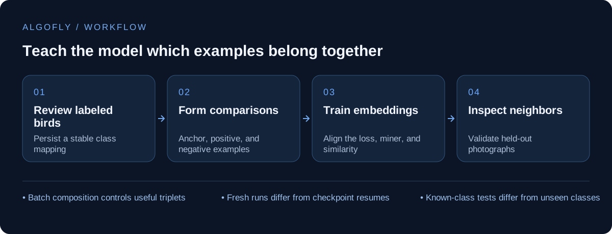
A triplet consists of an anchor, a same-class positive, and a different-class negative. The margin objective asks the model to favor the positive by a useful separation. The project uses PyTorch Metric Learning's cosine similarity, triplet-margin loss, and a semi-hard triplet miner with a margin of 0.2.
The miner chooses which relationships contribute to learning; it does not create missing positive examples in a batch. Include multiple instances per class often enough to form useful triplets, and track the number of selected triplets during training. A low loss accompanied by no useful comparisons is not evidence of a strong embedding.
This is an illustrative training-step outline using the project's components. The surrounding model, loader, optimizer, and device handling still need to be configured:
optimizer.zero_grad()
embeddings = model(images)
selected_triplets = mining_func(embeddings, labels)
loss = loss_func(embeddings, labels, selected_triplets)
loss.backward()
optimizer.step()
Keep the loss and miner's similarity configuration aligned. Distances and similarities have opposite ordering conventions, and changing one component without the other can invalidate the intended comparisons.
Separate a fresh run from resuming
The checked-in notebook includes a checkpoint-loading line before the training loop. That is useful when resuming an experiment, but a first run does not yet have that file. Decide explicitly whether you are starting fresh or resuming, rather than treating a missing checkpoint as a dataset problem.
The example also uses a large batch size and a CUDA device. Adapt those settings to the actual hardware and watch memory use during evaluation, when many embeddings may be held in memory. Reducing batch size changes which comparisons are available, so revisit sampling and mining behavior rather than viewing it only as a memory adjustment.
For an old experiment, record compatible package versions in an isolated environment. The repository's older torchvision construction syntax and dependency choices are useful historical context, but should be checked before use with a new PyTorch installation.
Validate neighbors as well as loss
The training loop evaluates the representation against reference embeddings and saves recent and best checkpoints. Inspect actual neighbor images at regular intervals. Are mistakes between visually similar species, or is the model matching backgrounds, framing, or color patches instead of the bird?
Report the exact query and reference sets used. A model evaluated on known species from held-out photographs answers a different question from a model evaluated on species absent from training. Neither result should be presented as the other. For an application with unknown inputs, add a rejection policy and test it with deliberately out-of-scope images.
Keep a small fixed set of queries for comparing checkpoints. That makes regressions visible even when the overall average changes only slightly. Also inspect classes with few examples: a strong aggregate can hide a subset that never receives useful training comparisons.
Move from a checkpoint to a search system
At the end of part one, the artifact is an image-to-vector function. A practical application still needs a gallery, metadata, search, and an update policy. Part two builds that layer with Qdrant and shows how a learned representation becomes a similarity-search workflow.