A general-purpose image model can recognize the subject of a picture while missing the distinction your application cares about. Two bird species may look almost identical to a broad semantic model; two views of the same species may have different poses and backgrounds. Our image embedding training video explores learning a representation for that narrower similarity problem.
The accompanying public project makes the experiment concrete. It prepares a bird dataset, fine-tunes a DINOv2-based vision transformer with Open Metric Learning, compares embeddings, and uses Qdrant for nearest-neighbor evaluation. This is a custom training workflow built on pretrained features, rather than training a vision transformer from random initialization.
Decide what a useful neighbor means
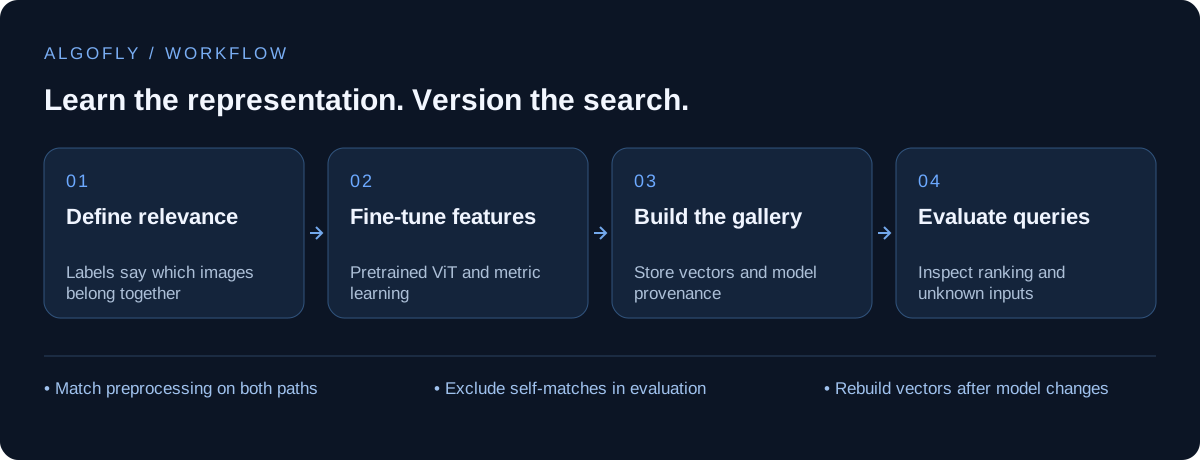
An embedding is a numeric representation used to compare images. The representation becomes useful when proximity agrees with the application's notion of relevance. For bird identification, a useful neighbor might be another photograph of the same species. For a product catalog, it might need to be the exact SKU, a matching variant, or a visually related alternative. Those are different targets.
Write that target down before choosing a loss or collecting labels. If red and blue packaging should count as the same product, the training pairs must communicate that. If color distinguishes variants, an augmentation that destroys color can work against the task. The data policy determines what the model is encouraged to ignore.
Follow the four notebooks
The repository separates preparation, training, inference, and evaluation into four numbered notebooks. That division is useful because each stage produces an artifact the next one consumes: a dataset manifest, a checkpoint, an embedding function, and an indexed gallery. Keeping those boundaries visible makes it easier to identify whether an error comes from data, training, or search infrastructure.
The checked-in preparation notebook uses CUB-200-2011 data and builds a CSV with image paths, labels, splits, and query/gallery flags. The training configuration selects a vitb14 extractor initialized from vitb14_dinov2, normalized features, and a triplet loss with hard-triplet mining. These are the repository's example choices; they are not requirements for every embedding application.
Make the split reflect the question
The example preparation code divides images within each species between training and validation. This supports evaluating recognition of known species from different images. It does not, by itself, establish performance on entirely unseen species. A class-disjoint split is needed if the intended question is whether the representation transfers to identities absent from training.
There is another detail worth checking before reproducing the experiment: the notebook marks validation records as both queries and gallery members. Retrieval evaluation must exclude the query image itself when those sets overlap. A near-perfect self-match says little about the quality of the remaining neighbors. Always document whether evaluation excludes exact duplicates and near-duplicate photographs.
For reproducible preparation, sort input file paths, choose a recorded random seed when shuffling, and persist the label mapping. The example contains a signed dataset download URL; obtain a fresh authorized dataset download instead of expecting an old temporary link to remain usable.
Why the sampler matters as much as the loss
A triplet contains an anchor image, a positive example of the same class, and a negative example from another class. The training signal encourages the positive to be closer to the anchor than the negative. A batch that contains only one image of each class may not provide the positive relationships this setup needs.
The repository addresses this with a balanced sampler configured for 25 labels and six instances per label. The same configuration uses AdamW with a learning rate of 1e-5 and a maximum of 200 epochs. Treat these as an inspectable starting recipe. Batch composition, available GPU memory, annotation noise, and dataset diversity should drive the final settings.
Hard mining focuses learning on difficult relationships. It can also amplify errors in the labels: two genuinely similar images assigned conflicting classes may repeatedly become hard negatives. Inspect hard examples during training instead of assuming that every difficult pair is useful supervision.
Keep preprocessing and the checkpoint together
The inference notebook loads a saved extractor checkpoint and obtains the matching pretrained transform from Open Metric Learning. The evaluation notebook additionally converts images to RGB and applies the project's resize-and-pad helper. This is an important place to standardize the implementation before deployment: gallery and query images should go through the same color conversion, geometry, normalization, and model mode.
The following example illustrates a basic comparison once an application has produced embeddings. It does not replace the repository's model-specific preprocessing:
import numpy as np

def normalized(vector):
    vector = np.asarray(vector, dtype=np.float32)
    norm = np.linalg.norm(vector)
    if norm == 0:
        raise ValueError("An embedding must have nonzero length")
    return vector / norm

# query_vector and gallery_vectors come from the same model version.
query = normalized(query_vector)
gallery = np.stack([normalized(v) for v in gallery_vectors])
scores = gallery @ query
best_indices = np.argsort(-scores)[:5]
This brute-force baseline is valuable even if production uses an approximate index. It provides a way to separate representation quality from indexing behavior on a manageable subset.
Evaluate retrieval and classification separately
The evaluation notebook indexes training images in a cosine-distance Qdrant collection and retrieves a nearest neighbor for validation images. Comparing the neighbor's label with the query label produces a top-one recognition measure. That is useful, but it does not describe every aspect of a search experience.
For a ranked gallery, measure whether relevant examples appear within the first few results and whether the ranking is dominated by duplicates. Review per-class errors and cases where no suitable match exists. If the application must reject unknown products or species, introduce a held-out unknown set and tune rejection behavior against it rather than treating any top result as an answer.
The video description discusses comparisons with CLIP, DreamSim, and ImageBind. Such comparisons are task-specific. A strong result on this bird experiment is not evidence that the custom model universally outperforms those models across every dataset or every definition of similarity.
Version the whole search system
A new checkpoint creates a new embedding space. Replacing the model while leaving old gallery vectors in place can produce meaningless scores even when the vector dimensions match. Version the model, transform, label map, and gallery together. Build a new collection, validate it with a fixed query set, and switch traffic only when the complete bundle is ready.
This workflow is useful beyond birds: domain-specific visual search, catalog matching, image deduplication, and inspection can all benefit from a representation trained around the right relationships. The first question remains the same: which images should be neighbors, and how will you know the ranking is useful?