
On 206 price-tag crops, WATERec rank-192 and PP-OCRv6 Medium each read 163 prices exactly. PP-OCRv6 Small read 160 and took just 0.60 milliseconds per crop on our RTX 5090. For a reader handling one tag at a time, that leaves a concrete choice: how much processing time are three additional correct prices worth?
I wanted a reader that could return one useful string from a crop. For a shop, that might be 10.95 DH. For a gate camera it might be AYO9034. A missing decimal can change what someone pays. A single wrong letter can point to a different vehicle. That is why I counted complete, exact strings. A six-character near miss earns the same zero as a blank prediction.
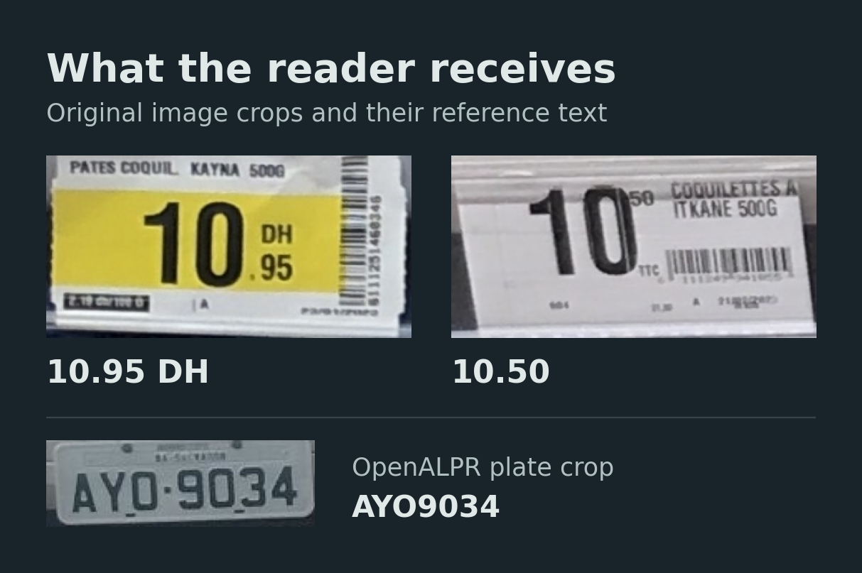
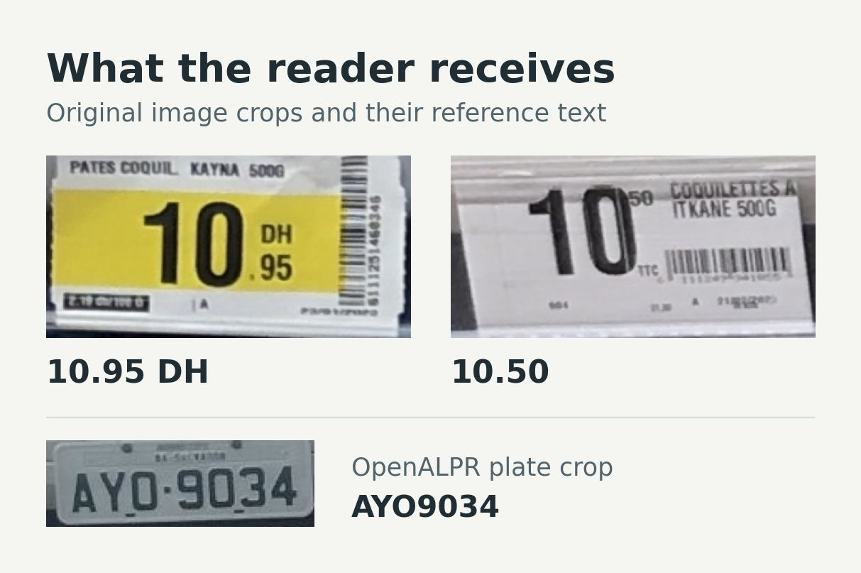
Look at the yellow tag first. Your eye lands on the large 10. The smaller 95 sits below DH, yet its label reads 10.95 DH. The reader has to join the whole amount, insert the decimal and put the currency after the cents. On the white tag the large digits also say 10. This time the small raised digits are 50 and the archive label is 10.50. Reading just the two most prominent digits gives the same answer for two different prices.
The plate presents a different transcription decision. Its printed separator is visible, while the benchmark reference joins the letters and digits as AYO9034. These labels give the training loop an answer to learn and the evaluator a string to compare. They also explain why we reviewed label conventions before comparing models. View the original OpenALPR photograph.

What went into the experiments
The plate experiments used a private collection with 10,990 training crops and 2,693 local validation crops. The 984 crops called “unseen plates” in our results came from a separate private evaluation set. We reused that set across experiments and scored complete registrations against AI-reviewed transcriptions. The public OpenALPR benchmark supplied a different, 443-crop international test. Its images and scores are counted separately. Plate fonts vary, glare erases strokes, and two-line registrations force a reader to decide which character comes next. In the PARSeq recipe I added 2,048 synthetic single- and two-line examples during training. The public notebooks include a tiny synthetic dataset so you can run the workflow. Reproducing the scores requires the training data and fitted checkpoints, which are private.
For prices, the report includes runs with 820 training images and a separate experiment limited to 50 labels. A 144-image internal holdout measures adaptation. A broader set of 206 corrected crops measures recognition on consistently framed tags, all 160 by 320 pixels at source. Of those references, 68 still carry provisional labels.
Reading the whole price tag
Look again at the two price crops above. A reader that returns just 10 misses both prices. In the figure below, a crop earns one correct read only when the entire prediction matches its reference, including the cents and any expected currency text.
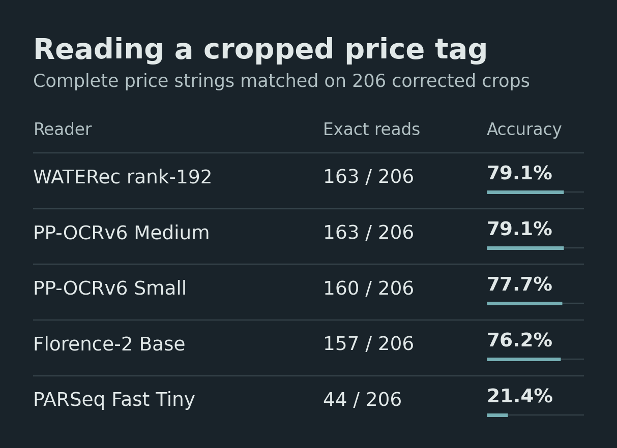
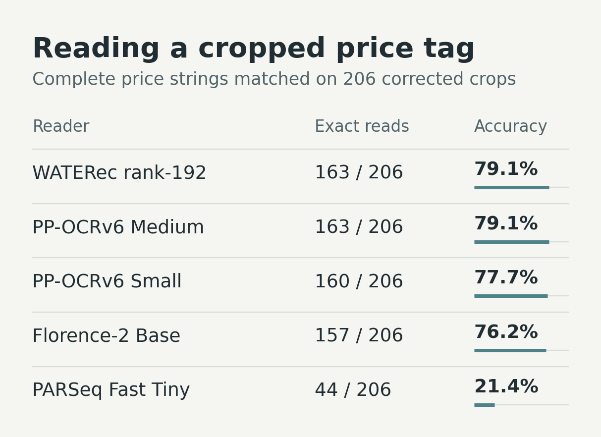
WATERec rank-192 approximately preserves the proportions of the input crop. Its paired-format head looks for the currency and separator in the image. PP Medium uses a fixed 128-by-320 input. The two readers reached the same exact-match count here. That tie alone cannot tell us whether they missed the same tags.
For an application that already supplies cropped tags, PP-OCRv6 Small is more attractive. It read 160/206 correctly in 0.60 ms per decoded crop on the RTX 5090. Medium bought three additional reads for 0.77 ms. WATERec rank-192 took 1.17 ms on those crops.
The gate camera test
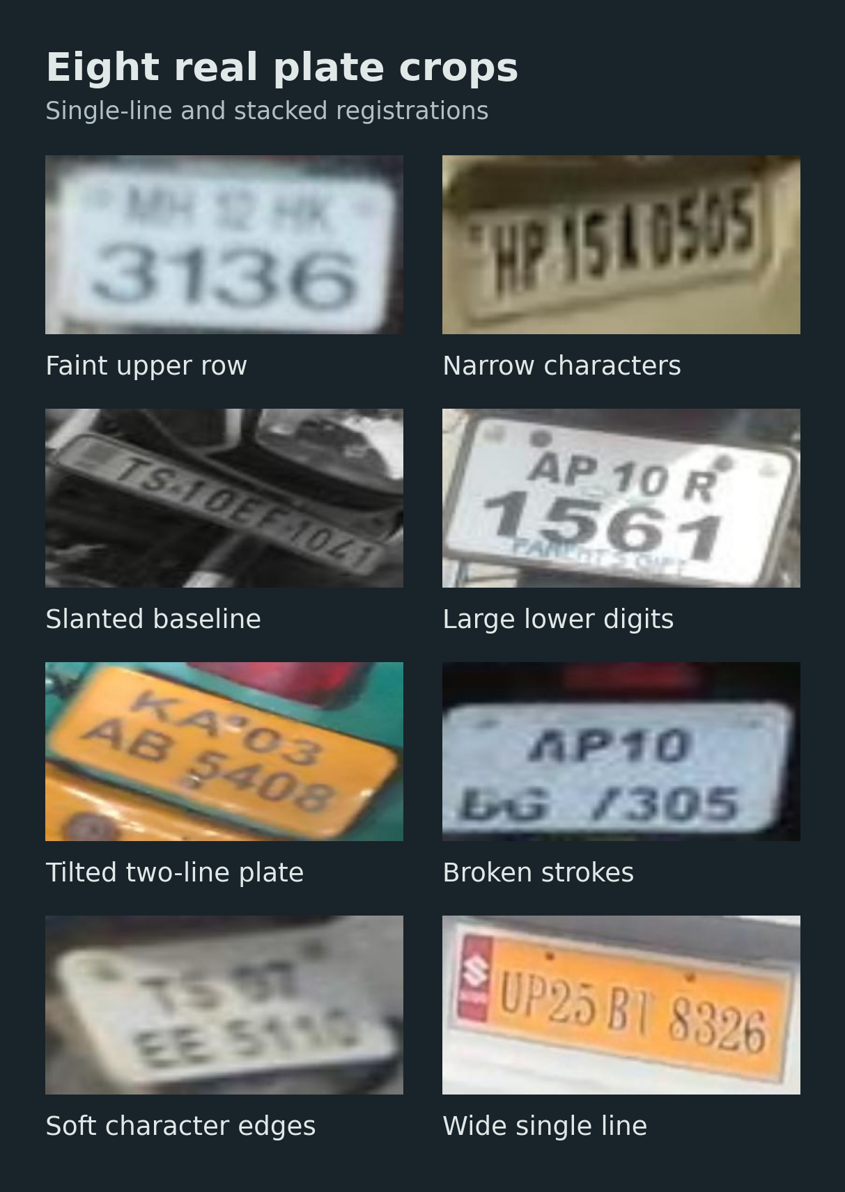
Start with the top-left crop. The four digits on the lower row are easy to pick out, while the characters above them nearly disappear. A reader that returns only the bottom row still loses the entire example under exact-match scoring. Now look at the slanted plate in the second row. Its characters sit on one diagonal line. Splitting every crop into a top and bottom half would cut through those characters. This mix of layouts explains why the PARSeq training recipe included both one-line and two-line examples.
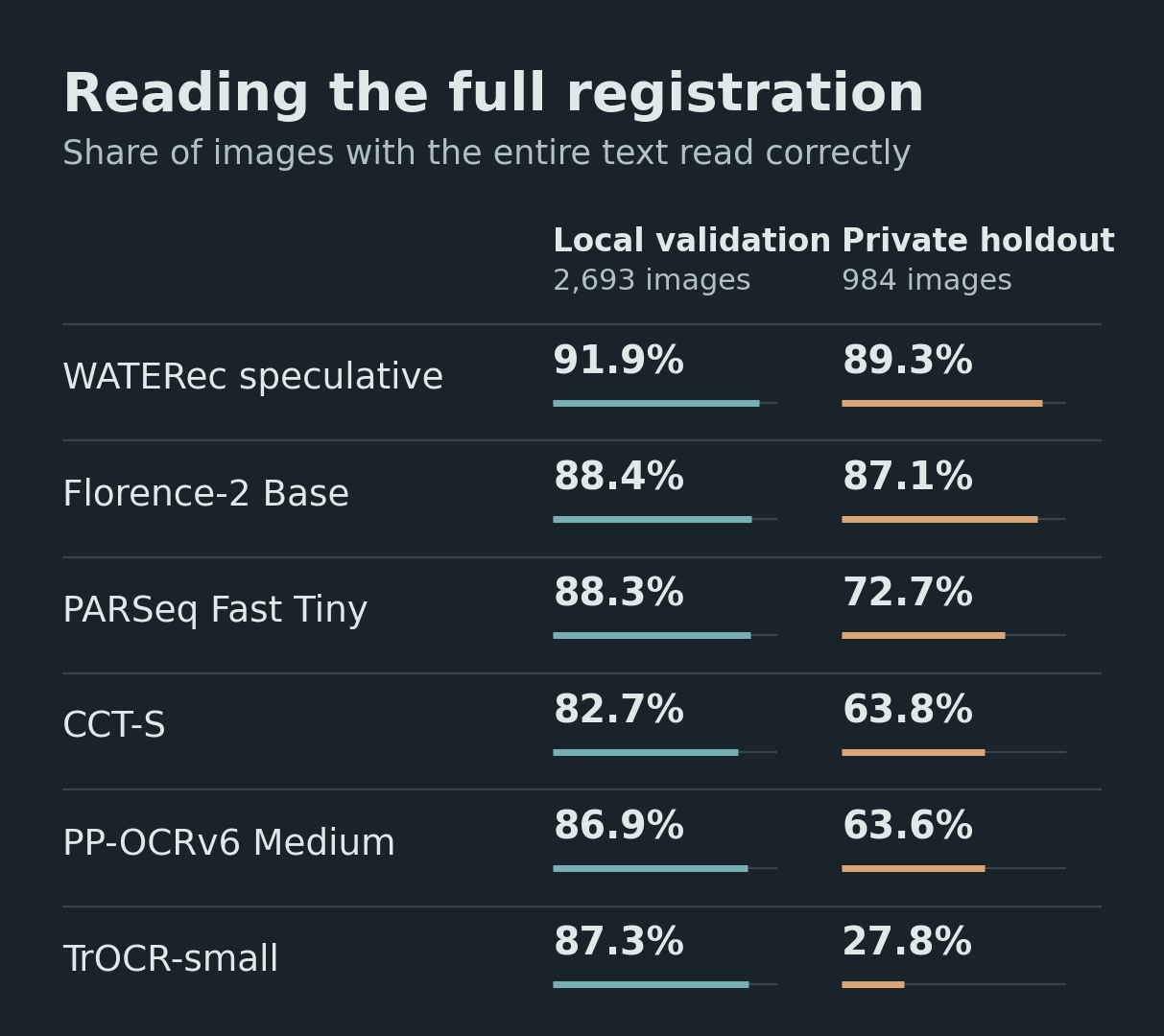
Florence-2 and PARSeq Fast Tiny were four plates apart on local validation, 2,381 versus 2,377 correct. On unseen plates the gap grew to 142 reads, 857 versus 715. TrOCR-small showed the steepest drop, from 2,350/2,693 locally to 274/984 unseen. I would want a second camera, a different location and a new plate format in my acceptance set before taking a local result to production.
My first pick for unfamiliar plates is the WATERec speculative profile. It read 879/984 correctly at 1.07 ms per decoded crop and 700 MiB sampled GPU memory. Florence-2 Base read 857 at 4.88 ms and 1,130 MiB on the same cohort. For a familiar lane with a tight latency budget, PARSeq Fast Tiny deserves a trial. Its 0.69 ms timing came from a separate workload, so I would time both engines on that lane before committing.
Distance changes the choice again. On 32 legible plates originally just 32–47 pixels wide, Florence read 14 directly, PARSeq 13 and WATERec 11. After 2× Lanczos resizing, WATERec reached 21, PARSeq 15 and Florence 13. Upscaling cannot recover a missing stroke, but it changes how the recognizer samples the strokes that remain. With only 31 distinct registrations this is a reason to try both input paths on your footage.
If I only had fifty labels
I gave each recipe the same 50 price images, 200 updates and batches of eight. On the separate 144-image holdout, tuning the decoder of generic Florence-2 produced 92 exact reads. Starting from a Florence checkpoint that had already learned plates raised that to 98. Generic WATERec decoder tuning returned 71, PP Medium with an auxiliary training objective returned 65, and a WATERec low-rank adapter returned 53. Limiting the adapter to 25,344 trainable parameters saved training capacity but cost 18 reads against WATERec decoder tuning.
For a new field with few labels, I would start with Florence and keep enough labelled examples aside to judge it. This was one seed, and equal update counts still leave different compute budgets and objectives. The speed figures above belong to separately trained deployment checkpoints.
What it took to make Tiny fast
Fast Tiny began with a 64-by-256-pixel reader. We trained it to predict characters in different orders, then taught it to propose a whole string in parallel and refine that proposal twice. During refinement it had to work with its own guesses. Giving it the correct prefix during training would hide precisely the mistakes it has to recover from at a gate.
Only then did we shrink the input to 48 by 192. We resized the learned position embeddings and mixed one synthetic letter-and-digit crop into every four real examples. To choose when to stop each stage, we held labels apart inside the training split. A separate run refitted on the full training set for the selected number of epochs. The external plates stayed available for the question that mattered later: would that smaller reader still work on somebody else’s camera?
What changes when the checkpoint becomes an engine?
Training produces weights. Native inference runs those weights through the framework used to develop the model. In the PARSeq workflow, ONNX is the exported graph and TensorRT builds an engine for deployment. Each step gives us another opportunity to change a prediction. We therefore check the returned text as well as the stopwatch. A portable graph by itself tells us nothing about how fast a particular runtime will execute it.
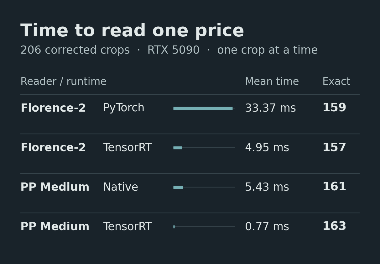
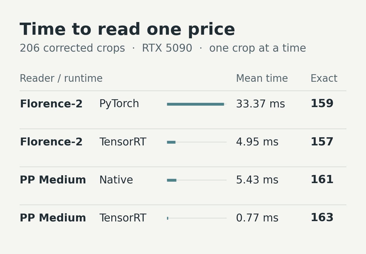
On 206 corrected prices, Florence went from 1,768 MiB of GPU memory in native PyTorch to 1,452 MiB with optimized TensorRT. PP Medium went from 724 to 656 MiB. Both became roughly seven times faster on decoded crops. Their exact counts moved in opposite directions. Two fewer correct reads can conceal several individual gains and losses, so the export check worth keeping is the per-image disagreement list.
Precision deserves its own control. On the separate 144-tag development set, PP Medium’s mixed TensorRT engine and its full-FP32 control both read 104 prices correctly. Mixed precision took 0.884 ms from RGB versus 1.413 ms for FP32, yet used more sampled process memory, 654 versus 588 MiB. The training recipe used 676 fitting images for this development comparison. Forty-five of the 144 references still had unresolved visual ambiguity. Keep the denominator, the precision and the label policy beside the score.
One shopper waiting, or eight crops already queued?
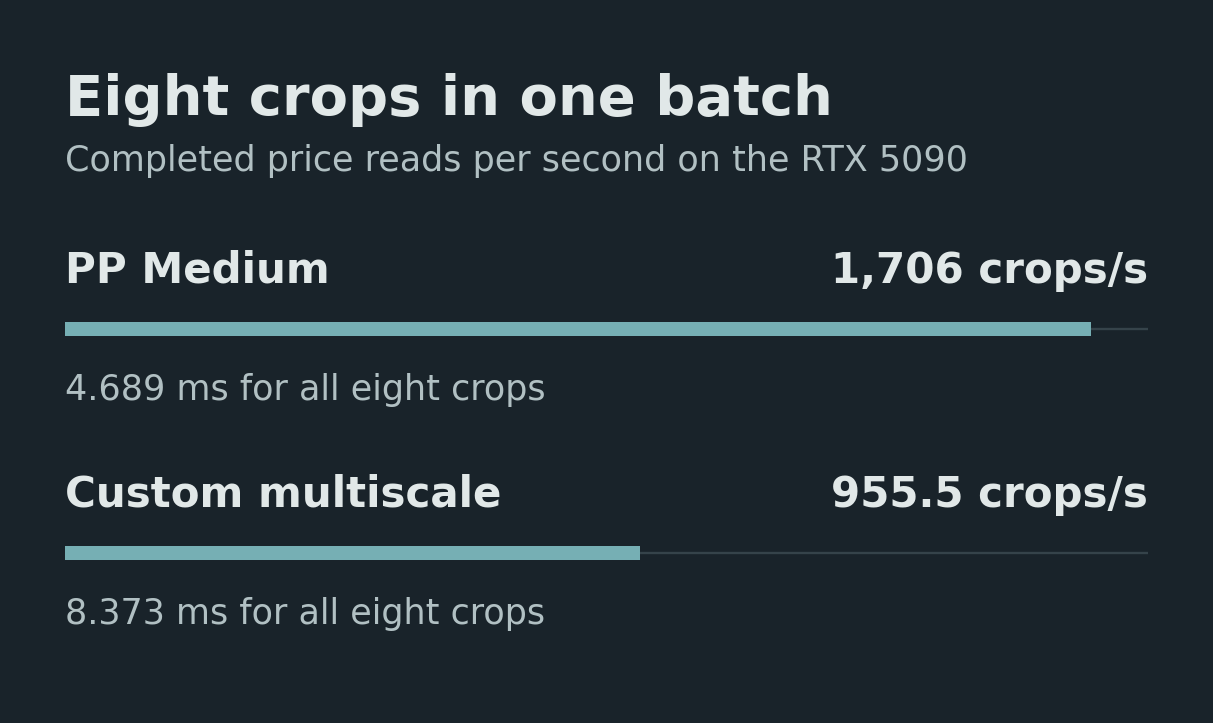
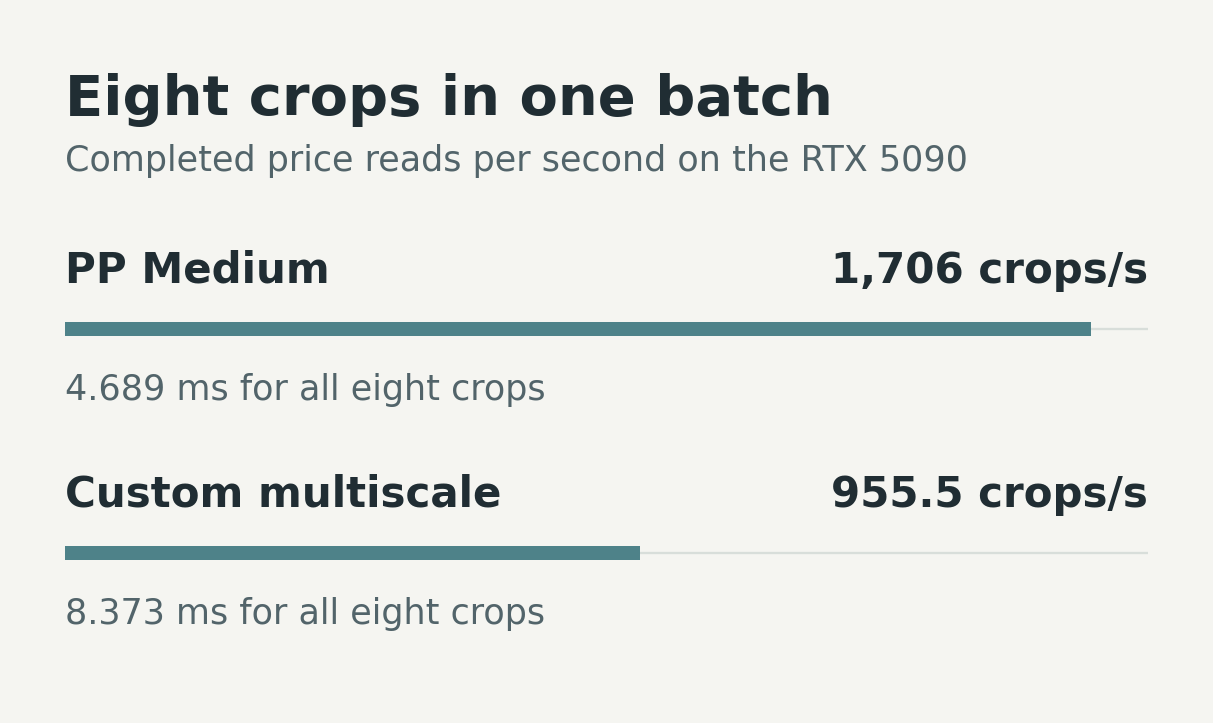
PP Medium processed eight decoded crops in 4.689 ms, about 1,706 crops per second. Dividing by eight gives 0.586 ms of amortized work per crop. A shopper waiting for one result still waits for the batch to fill and run. The custom multiscale reader took 8.373 ms for eight crops, or 955.5 crops per second. These are measured fixed-resolution runs on an RTX 5090. They answer a warehouse queueing question much better than a single-camera response-time question.
We checked all 144 price strings at each supported batch capacity, one, two, four and eight. PP kept its 104 exact matches across capacities, although three frame-level sequences changed and its strict numerical check failed. Repeated character predictions can collapse to the same final price. For an application that bills from the text this distinction matters differently than for one that consumes per-frame confidence.
There is also a historical same-protocol plate comparison for readers choosing a base model. Fine-tuned PARSeq TensorRT reached 941 crops/s at batch 32 against 376 for Florence-2 TensorRT. At batch one their median latencies were 4.00 and 9.12 ms. The recorded native-to-engine validation scores were 89.75% to 89.68% for PARSeq and 88.34% to 88.04% for Florence. Those older scores use the historical evaluation protocol. The current audit leaves PARSeq Base’s literal-output score unverified. There is no matched ONNX Runtime speed measurement for those rows. Inspect the backend measurements, batch qualifications and precision checks.
Which reader would I train first?
| Job | First trial | What would decide it |
|---|---|---|
| Clean, repeated price layout | PP-OCRv6 Small | Try Medium if three extra exact reads per 206 justify the latency on your device. |
| Plates across cameras | WATERec speculative | Review every wrong full registration. Try 2× resizing on naturally tiny crops. |
| Familiar lane, fast reads | PARSeq Fast Tiny | Test a new camera before accepting the local 88.27% result. |
| Very small model footprint | CCT-S | 0.98M parameters and 628/984 unseen plates. Check whether that error rate is affordable. |
| New price field, few labels | Florence-2 Base | Compare generic and domain-trained initialization on untouched examples. |
| Existing TrOCR installation | Keep TrOCR-small as a baseline | Replay unfamiliar plates before investing in its runtime. |
From an RTX workstation to a Jetson
The measured desktop reference was an RTX 5090 running one crop at a time. For an edge prototype with one camera and a modest recognition rate, I would try PP Small or PARSeq on a Jetson Orin Nano 8 GB. For a detector and WATERec sharing a device, I would start the capacity test on an Orin NX 16 GB. An AGX Orin is a candidate when several streams or other models share memory. Those are proposed trials. The reported experiments establish desktop timings only. NVIDIA’s Orin module specifications.
Count crops before buying hardware. Four cameras sampled at ten frames per second with three tags per frame generate 120 recognition requests per second. Replay a busy minute on the intended board, build the TensorRT engine for its installed software, and compare its output strings with the reference model. Time capture, detection, crop extraction and decoding through to the final text. Record the 95th-percentile delay, dropped frames and total shared memory after the board warms up. A 700 MiB GPU process peak on a desktop leaves all those other costs to pay.
Train on your own crops
Save a crop and its literal target string as a pair. Write down how to handle leading zeros, currency and stacked rows before labelling. Hold out a whole camera or store, then look at its misses alongside the image. If the detector cut off the cents, collecting a better crop is a more promising next experiment than adding decoder parameters.
Start with the benchmark snapshot, protocols and PARSeq notebooks. The other training repositories are WATERec, PP-OCRv6, Florence-2 and CCT. Keep the recipe and checkpoint alongside every score.